Excel is a strong tool that can assist you in many ways with data organization and analysis. The XLOOKUP function in Excel is among its most crucial features. You can use this flexible tool to look up a specific value in a group of cells and have the corresponding value from another column returned. In Excel 2019 and later versions, the XLOOKUP function was added as a new feature. Due to its adaptability and simplicity of use, XLOOKUP in Excel has quickly become one of the most used functions for data analysis and manipulation.
Key Takeaways:
- XLOOKUP replaces older lookup functions like VLOOKUP and HLOOKUP with simpler syntax and more flexibility.
- It can search in any direction—left, right, up, or down—unlike VLOOKUP.
- Exact match is the default, but it supports approximate matches, wildcards, and case-sensitive lookups (with help from EXACT).
- It can return multiple values (spill results) instead of a single cell value.
- Optional arguments allow custom “not found” messages, last-occurrence lookups, and more advanced search modes.
Follow the step-by-step tutorial below and make sure to download the Excel workbook to follow along:
Now that you are comfortable with the syntax of this incredible function, let’s dive into a few examples to understand how to use Excel XLOOKUP!
XLOOKUP – An Introduction
What does it do?
Excel XLOOKUP can be used to search an array for a specific value and returns the value in the same row from another array.
- It can search the value both horizontally and vertically,
- Perform an exact or approximate match,
- Use wildcards,
- Return a custom text when no result is found,
- Doesn’t even have the restriction of the return array to be on the right of the lookup array.
Isn’t that AMAZING? It is a power-packed function with so many advantages!
Formula breakdown
=XLOOKUP (lookup_value, lookup_array, return_array, [if_not_found], [match_mode], [search_mode])
where:
- lookup_value – the value you want to search;
- lookup_array – the range or array where you want to search the value;
- return_array – the range or array from which you want the result;
- [if_not_found] – the value you want to display if there are no results found;
- [match_mode]
- 0 – Exact Match (if no result found, then error)
- -1 – Exact or next smaller (if no result found, then the next smaller value will be displayed)
- 1 – Exact or next larger (if no result found, then the next larger value will be displayed)
- 2 – Wildcards
- [search_mode]
- 1 – to search from first
- -1 – to search from last
- 2 – binary search ascending
- -2 – binary search descending
Advantages of XLOOKUP
XLOOKUP is a versatile and outstanding replacement for the above-mentioned Excel functions. It allows you to quickly lookup values in a data set (just like VLOOKUP Excel) with additional flexibility and advantages like:
- It can lookup data to the right or left of the lookup values.
- It looks for an exact match by default. You do not have to enter an additional argument for it.
- It allows you to provide a custom value or text if your search result is not found.
- It can perform a partial match lookup using wildcards.
- It can search for values both horizontally and vertically.
- It can return a range instead of a single value which spills out the results.
- It allows you to find the last occurrence in your data.
How to use XLOOKUP in Excel
Step-by-Step Guide
In this example below, there are two tables:
- Stocklist containing the product’s SKU, name, price, and cost.
- Orders Table with its quantity mentioned
You want to extract the price of the products from the stock list table using XLOOKUP.
STEP 1: We need to enter the XLOOKUP function in a blank cell
=XLOOKUP(
STEP 2:Enter the first XLOOKUP argument – Lookup_value (product’s SKU that you are looking for)
=XLOOKUP(H10,
STEP 3: Enter the second XLOOKUP argument – Lookup_array (the array that contains all product SKUs)
=XLOOKUP(H10,$E$9:$E$12
Ensure that you press F4 so that you can lock the table range
STEP 4: Enter the third XLOOKUP argument – return_array (the array that contains price)
=XLOOKUP(H10,$E$9:$E$12,$C$9:$C$12)
As you will see, Excel has pulled the price of the SKU LP1411 from the stock list and provided the result ($185) in the cell.
Apply the same formula to the rest of the cells by dragging the lower-right corner downwards.
What if you are trying to search for a product name that is not available in the stock list table?
Excel will provide you with an error!
Instead of showing this error, you can add a custom text (say, No Product Found) to display!
To do that, simply can add the fourth optional argument of XLOOKUP function – [if_not_found]
=XLOOKUP(H10,$E$9:$E$12,$C$9:$C$12,“No Product Found”)
This was a basic example of how to use XLOOKUP in Excel. Let’s explore the advanced uses of this function in detail!
Advanced Uses of XLOOKUP
Approximate Match
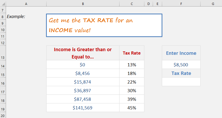
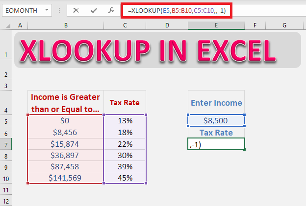
In this example, Excel will look for the income entered in cell F14 and find the matching tax rate from column C.
Instead of looking for an exact match, it will now look for an approximate match i.e. if an exact match is not found it will look for the next smaller or larger item based on the input provided.
If the income is greater than or equal to $0, the tax rate will be 13%. Similarly, if the income is greater than or equal to $8,456, the tax rate will be 18%, and so on.
So, let’s use this function to determine the tax rate for the income amount mentioned in cell F14.
=XLOOKUP (lookup_value, lookup_array, return_array, [if_not_found], [match_mode], [search_mode])
Here, the three permanent arguments and one optional argument [match_mode] will be used. You can ignore arguments – [if_not_found] and [search_mode] for this example.
Follow the step-by-step tutorial below to perform an approximate match using the XLOOKUP function:
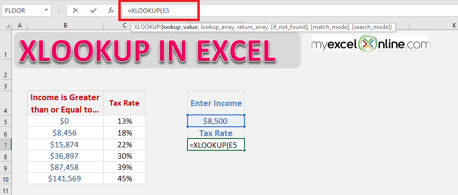
STEP 1: Enter the first argument lookup_value i.e. the income amount mentioned in cell E5.
=XLOOKUP(E5
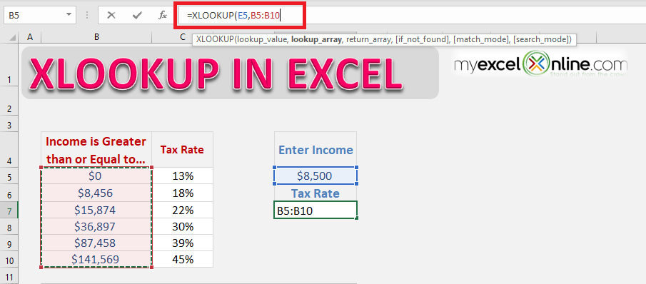
STEP 2: Enter the lookup_array i.e. the range containing income range (B5: B10).
=XLOOKUP(E5,B5:B10
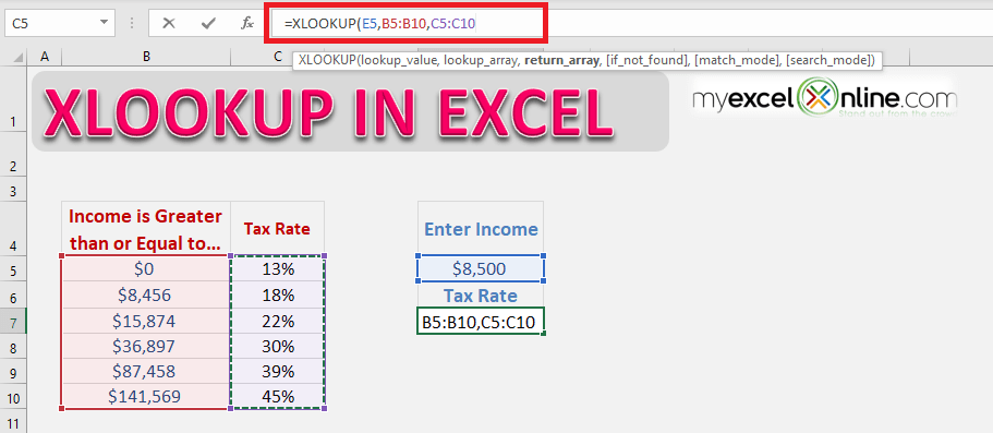
STEP 3:Enter the return_array
=XLOOKUP(E5,B5:B10,C5:C10
STEP 4: Enter the 5th argument[match_mode]. The accepted values for this argument are:
- 0 – Exact Match (if no result found, then error)
- -1 – Exact or next smaller (if no result found, then the next smaller value will be displayed)
- 1 – Exact or next larger (if no result found, then the next larger value will be displayed)
- 2 – Wildcards
In this example, the value will be -1.
=XLOOKUP(E5,B5:B10,C5:C10,,-1)
(Ignore the 4th argument)
Below is the formula that should be used:
=XLOOKUP(E5,B5:B10,C5:C10,,-1)
As you know this function will perform an exact match by default, you need to use the optional part of the function – [match_mode]. So, if Excel fails to find an exact match, it will look for the next smaller income range mentioned in the table.
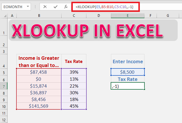
One of the advantages of using this function over Excel VLOOKUP for an approximate match is that you do not need to sort the data in ascending order. Excel will do that on its own!
In the example below, you will see that the data is not arranged in ascending order.
You can use the same formula in randomly arranged data and Excel will provide you with the same (correct) result.
Horizontal Lookup
The syntax for performing a horizontal lookup using XLOOKUP is the same as for vertical lookup.
You just need to provide Excel with the lookup and return an array, the table’s orientation is irrelevant to the XLOOKUP function.
In this example, the product name is displayed on Row 5 and the price is displayed on Row 6. You need to perform a horizontal lookup to get your results.
STEP 1: Enter the lookup value i.e. the product name mentioned in cell H6.
=XLOOKUP(H6
STEP 2: Enter the lookup array i.e. the array containing the product name.
=XLOOKUP(H6,$C$5:$F$5
STEP 3: Enter the return array i.e. the array containing prices of the product.
=XLOOKUP(H6,$C$5:$F$5,$C$6:$F$6)
It’s that easy to do a horizontal lookup using the new XLOOKUP function in Excel!
Return a Range instead of Value
Excel XLOOKUP has the ability to return multiple values instead of just one for a correct match. It can be done without making any change in the syntax, simply input the entire range in the function instead of just a single column or row.
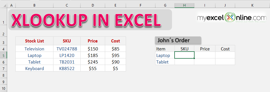
In this example, we want to retrieve all the details related to the product name mentioned in cell G5.
STEP 1: Select the cell containing the lookup value.
=XLOOKUP(G5
STEP 2: Select the range containing the product list.
=XLOOKUP(G5,$B$4:$B$7
STEP 3: Select the entire range containing columns for SKU, price, and cost.
=XLOOKUP(G5,$B$4:$B$7,$C$4:$E$7)
Excel will extract or “spill” all the values with the help of the XLOOKUP formula!
Using Wildcards
Xlookup in Excel allows you to search for a partial match using wildcards characters like: * ? ~
This can be done using Excel VLOOKUP as well. But the problem arises when you are actually trying to search the wildcard character itself in the data.
For XLOOKUP, you can use wildcards in the lookup_value argument and specify that in the [match_mode] argument. Enter 2 as the match_mode value to let Excel know that you are trying to do a partial match.
The three wildcards in Excel are:
- Asterisk mark (*) represents any number of characters. For example, Jo* could mean Joanne, John, Joe, etc.
- Question mark (?) represents one character. For example, Jo?n could mean John, Joan, etc.
- Tilde (~) can be used when you want the asterisk or question mark to not be a wildcard. Simply place a tilde just before * or ?.
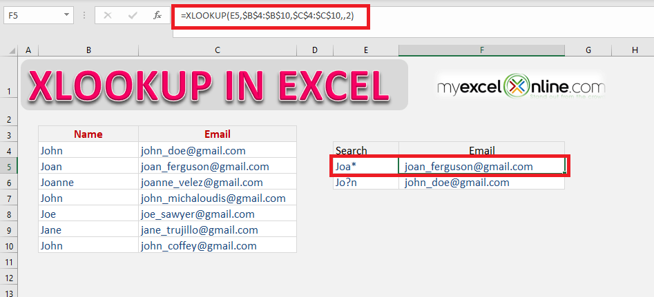
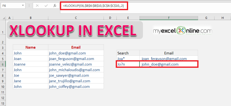
In these examples below, you can use wildcard characters (* or ?) to search for a partial match and return the corresponding email address.
Joa* will search for the first match starting with Joa and any number of characters after that (Joan) and return the corresponding email address ([email protected]).
=XLOOKUP(E5,$B$4:$B$10,$C$4:$C$10,,2)
Jo?n will search for the first match starting with Jo followed by one character and then n (John) and return the corresponding email address ([email protected]).
=XLOOKUP(E6,$B$4:$B$10,$C$4:$C$10,,2)
Search from bottom to top
In this example, we will search the value from bottom to top instead of the default direction (top to bottom). This can be achieved by using the 6th argument of the function – [search_mode].
It is an amazing feature if you wish to find the last occurrence of something in your data. Let’s dive into this XLOOKUP example to learn how.
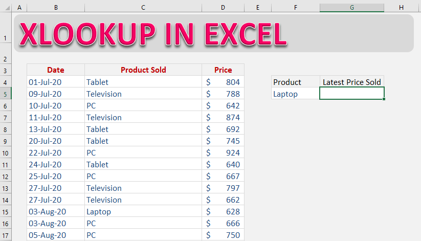
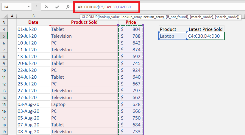
In this example, you have sales data with the Sales date, Product name and Price mentioned. You have to find out the latest price at which a particular product was sold.
Follow the step-by-step tutorial to search value from bottom to top:
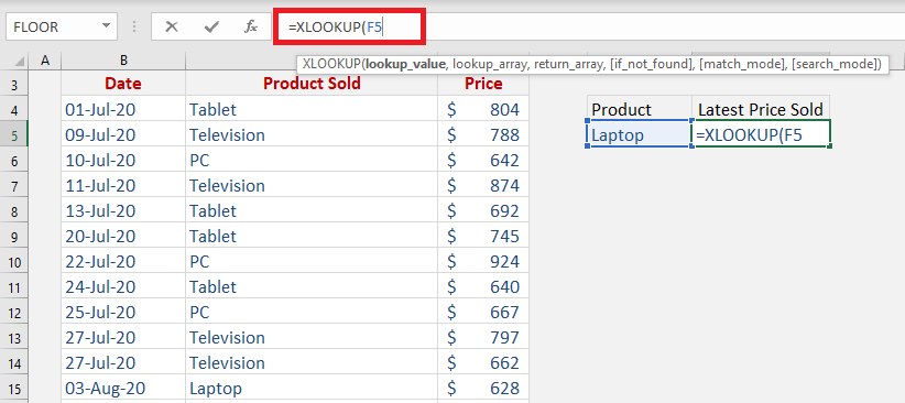
STEP 1: Enter the lookup value i.e. the product name mentioned in cell F5.
=XLOOKUP(F5
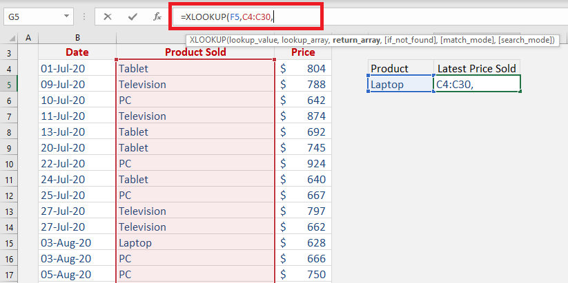
STEP 2: Enter the lookup array i.e. the array containing the product name.
=XLOOKUP(F5,C4:C30
STEP 3: Enter the return array i.e. the array containing prices of the product.
=XLOOKUP(F5,C4:C30,D4:D30
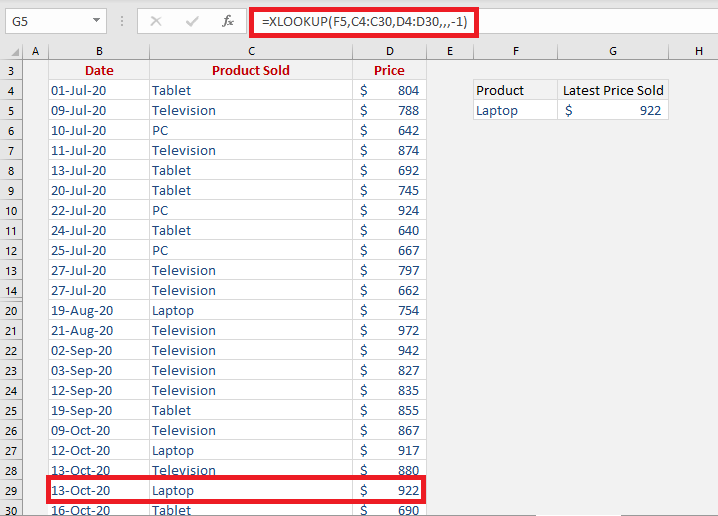
STEP 4: Enter the 6th argument [search_mode]. It will be -1 for this example as you want to search from bottom to top.
=XLOOKUP(F5,C4:C30,D4:D30,,,-1)
Excel will start the search from the bottom and the first match will be produced as a result!
Multiple spill values
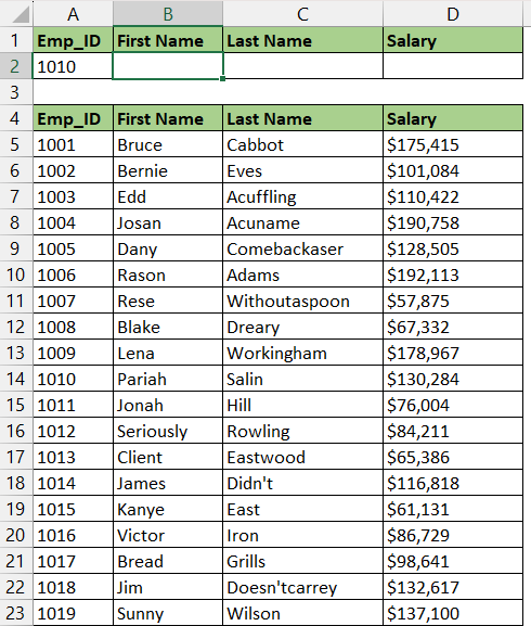
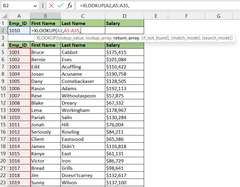
In this example, we have an employee ID mentioned in cell G1. We want to extract first name, last name, and salary based on the employee ID.
Let us understand the syntax here:
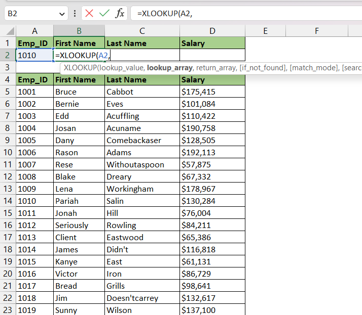
STEP 1: Enter the first argument – Lookup_value. Here our lookup value is in cell A2, which contains the employee id whose details we want to find out.
=XLOOKUP(A2,
STEP 2: Enter the second argument – Lookup_array. Here we are going to search in the column containing the list of employee id, i.e., A5:A35,
=XLOOKUP(A2,A5:A35,
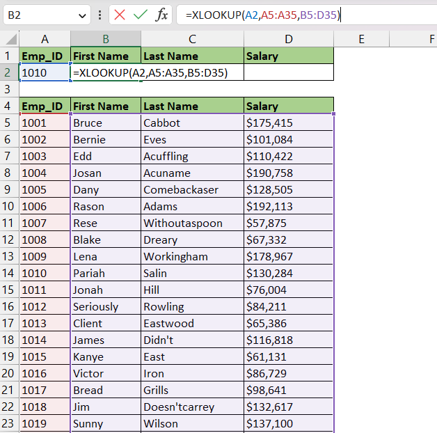
STEP 3: Enter the third argument – Return_array: Here we are going to select the columns containing the corresponding details such as first name, last name, and salary that we want to extract, i.e., B5:D35
=XLOOKUP(A2,A5:A35,B5:D35)
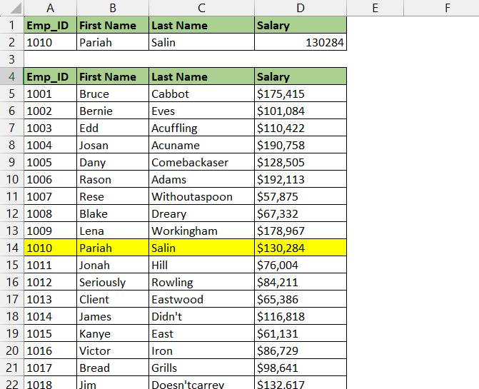
Here we have our employee id of 1010, which spills its corresponding values of the first name, last name, and salary. This is happening because we have selected 3 columns in the return_array argument.
Grid lookup
We can perform a Grid lookup by using nested XLOOKUP in Excel, i.e., using an XLOOKUP function inside another. As Excel works by solving the inner function first, the inner XLOOKUP function will be solved first.
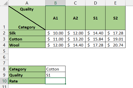
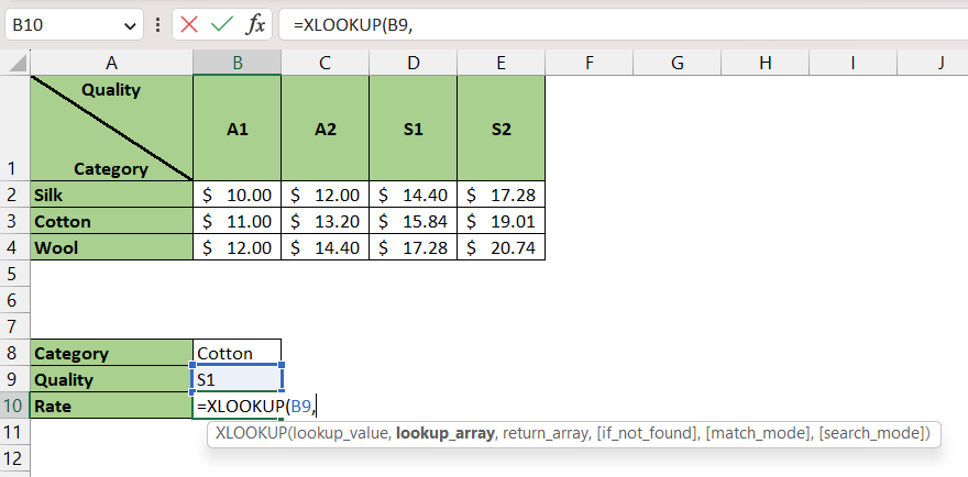
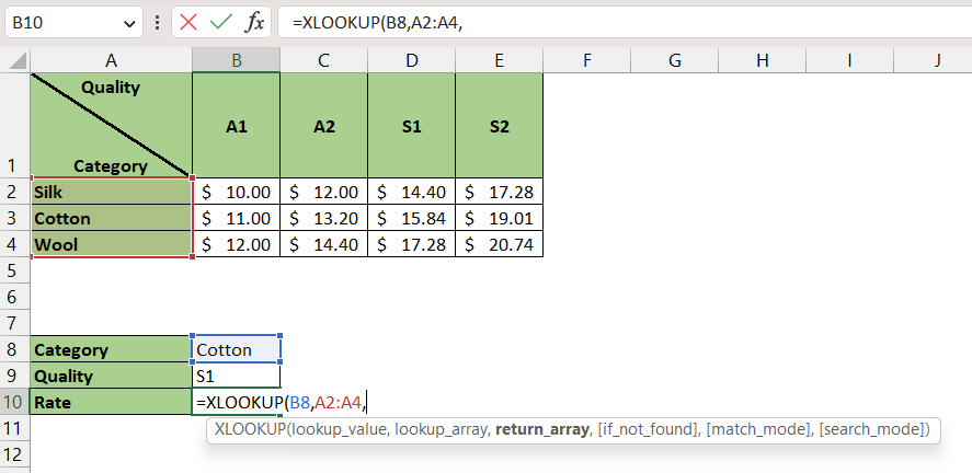
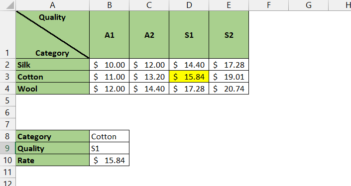
In this example, we are trying to get the rate for the category mentioned in cell B8 and the quality mentioned in cell B9. The inner XLOOKUP in Excel will be used to get the rate for the quality mentioned in cell B9 and then using the resultant array the rate for the category mentioned in cell B8 we will get the desired rate.
Let us understand the syntax of the inner XLOOKUP in Excel:
STEP 1: Enter the first argument – Lookup_value. Here our lookup value is in cell B9, which contains the Quality of the product that we want.
=XLOOKUP(B9,
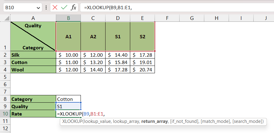
STEP 2: Enter the second argument – Lookup_array: Here we are going to search in the column containing the list of different quality levels offered, i.e., B1:E1
=XLOOKUP(B9,B1:E1,
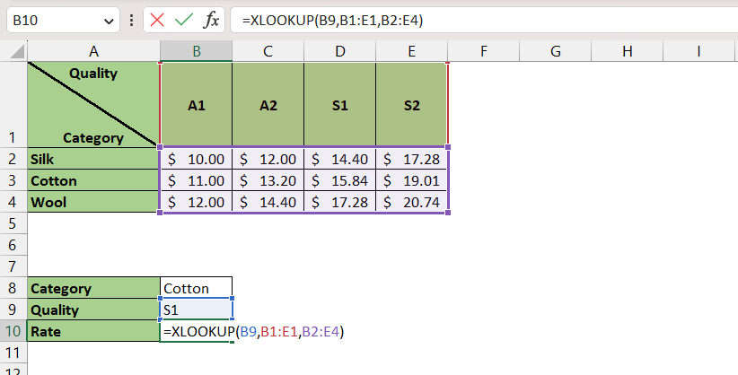
STEP 3: Enter the third argument – Return_array. Here we are going to select the entire array of prices, i.e., B2:E4
=XLOOKUP(B9,B1:E1,B2:E4)
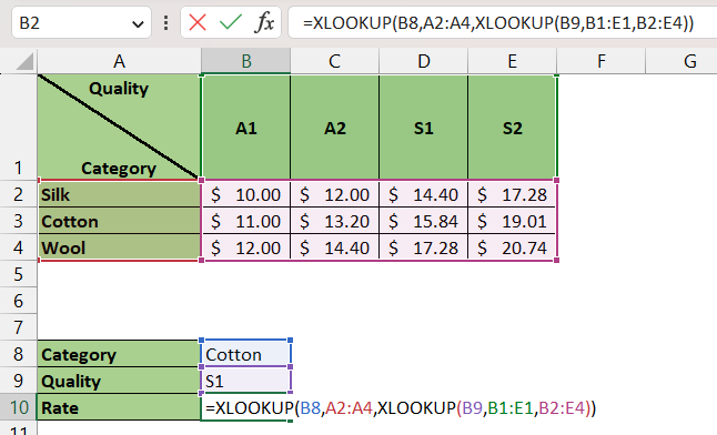
This XLOOKUP function will solve to give a spilled result of all the prices in column D, as we have observed earlier in our example. This result (D2:D4) is fed as result_array for the outer XLOOKUP in Excel. Let us understand the syntax here:
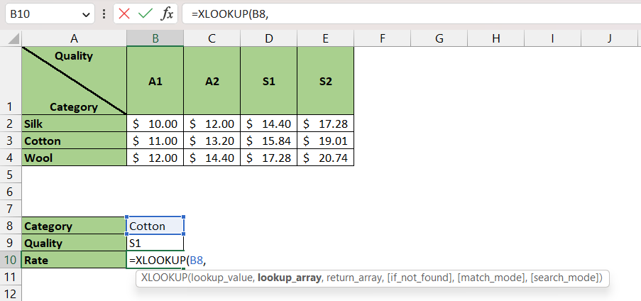
STEP 1: Enter the first argument – Lookup_value. Here our lookup value is in cell B8, which contains the Category of the product that we want.
=XLOOKUP(B8,
STEP 2: Enter the second argument – Lookup_array. Here we are going to search in the column containing the list of different categories of products offered, i.e., A2:A4
=XLOOKUP(B8,A2:A4,
STEP 3: Enter the third argument – Return_array. Here we will be adding the inner XLOOKUP in Excel.
=XLOOKUP(B8,A2:A4,XLOOKUP(B9,B1:E1,B2:E4))
This XLOOKUP in Excel matches the category of product desired and gives the corresponding price. The end result is the price of the category of product desired with the specified quality level.
XLOOKUP to the left
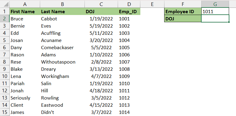
One major drawback of VLOOKUP was that it compulsorily had to keep the lookup array in the leftmost column of our dataset for it to be able to search for any criteria. Since XLOOKUP in Excel has separate arrays for both lookup and result, we can bypass this constraint and search right to left as well.
Let us understand the syntax here:
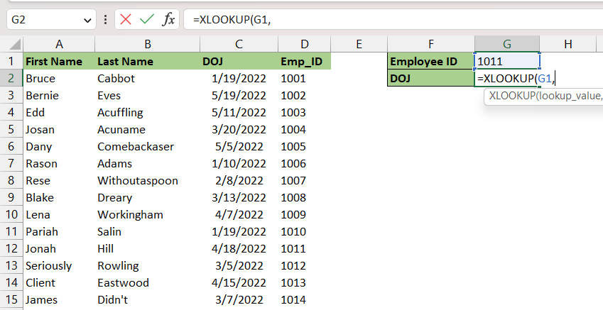
STEP 1: Enter the first argument – Lookup_value. Here our lookup value is in cell G1, which contains the employee ID.
=XLOOKUP(G1,
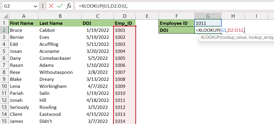
STEP 2: Enter the second argument – Lookup_array. Here we are going to search in the column containing the list of employee id, i.e., D2:D32
=XLOOKUP(G1,D2:D32,
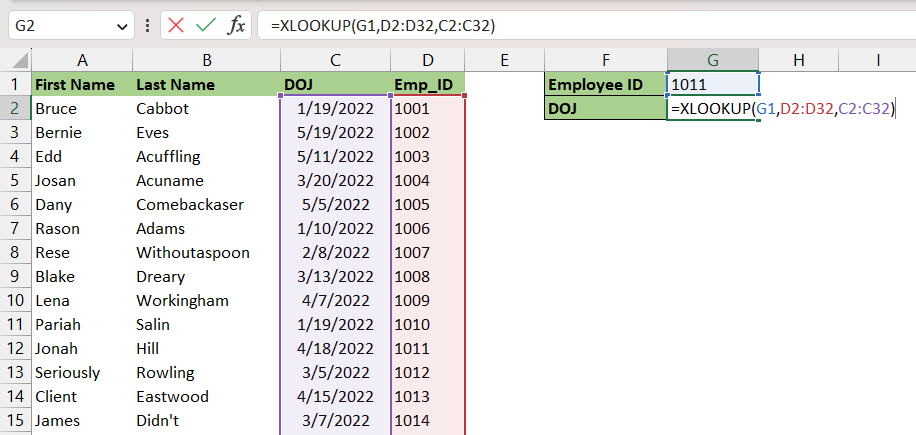
STEP 3: Enter the third argument – Return_array. Here we are going to select the entire array of corresponding date of joining of employees, i.e., C2:C32
=XLOOKUP(G1,D2:D32,C2:C32)
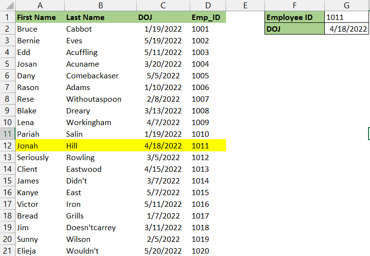
The salary for the mentioned employee ID has been returned by the XLOOKUP function in Excel even though the return array is on left of the lookup array.
Case sensitive XLOOKUP
The XLOOKUP in Excel is not case sensitive i.e. it treats both uppercase and lowercase as the same words. You can make XLOOKUP case-sensitive by using the EXACT Formula in Excel along with XLOOKUP.
The syntax of the EXACT function is –
=EXACT(text1, text2)
What it means:
=EXACT(first text to be compared, second text to be compared)
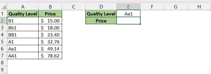
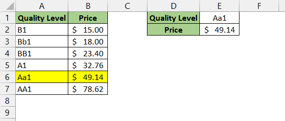
In this example, we are trying to exact the price for the quality mentioned in cell E1 using the list of quality and prices mentioned in the array A2:B7.
Let us follow the step-by-step tutorial below –
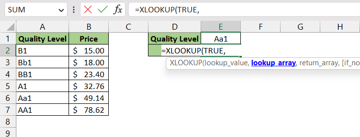
STEP 1: Enter the first argument – Lookup_value. Here our lookup value is TRUE, we are searching for an exact case-sensitive match. This function here works in tandem with the EXACT function.
=XLOOKUP(TRUE,
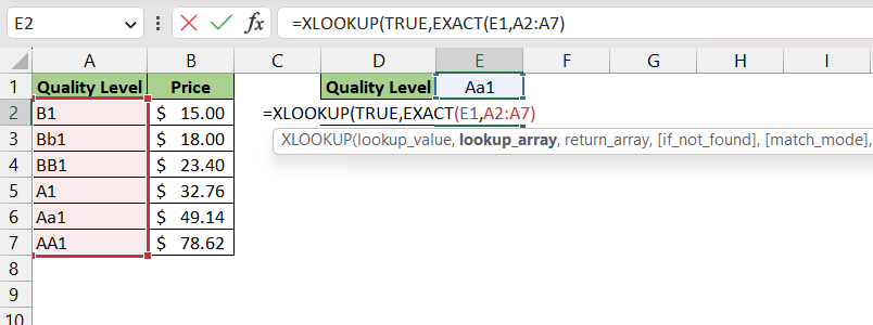
STEP 2: Enter the second argument – Lookup_array. Here we are using the EXACT function to compare the value in E1 (which contains the Quality level) to each cell in the range A2:A7 (list of all levels of quality offered). The EXACT function returns TRUE if the two numbers are exactly the same, and FALSE otherwise.
=XLOOKUP(TRUE,EXACT(E1,A2:A7)
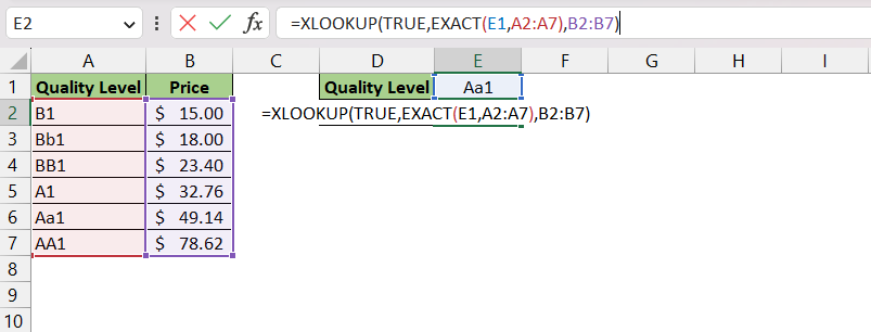
STEP 3: Enter the third argument –Return_array. Here we are going to select the entire array of the corresponding price of the product at different quality levels, i.e., B2:B7
=XLOOKUP(TRUE,EXACT(E1,A2:A7),B2:B7)
In this case, the XLOOKUP function searches for the first TRUE value in the array that the EXACT function has returned. If it discovers a TRUE result, it returns the value from the range B2:B7.
We can see that Excel has extracted the price of Aa1 i.e. $49.14 and not the price of quality AA1. Hence, allowing lookup to find case-sensitive values.
Multiple Criteria in XLOOKUP
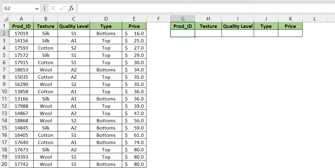
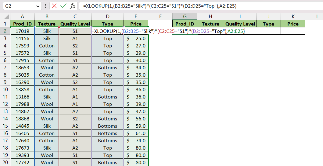
In this example, we will be searching for a value that matches more than 1 criteria using XLOOKUP.
Here, we are trying to get data for a product that matches the following three conditions –
- Texture is Silk
- Quality is S1
- Type is Top
Let us follow the steps below to understand how this can be accomplished.
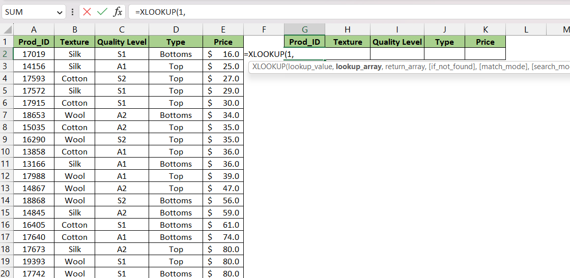
STEP 1: Enter the first argument – Lookup_value. Here our lookup value is 1. This is because test arrays will return 1 only when all the criteria are met.
=XLOOKUP(1,
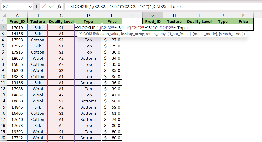
STEP 2: Enter the second argument – Lookup_array. Here we are checking multiple criteria. We will call them our test arrays.
- First, we want to extract details for a Silk product. We are searching for matches of “Silk” in the entire array B2:B25.
- Then we want a product of the S1 quality category. We are searching for matches of “S1” in the entire array C2:C25
- Finally, we want the details of a Top product. We are searching for matches of “Top” in the entire array D2:D25.
=XLOOKUP(1,(B2:B25=”Silk”)*(C2:C25=”S1″)*(D2:D25=”Top”)
STEP 3: Enter the third argument – Return_array. Here we are going to select the entire array because we want to extract the entire details of the product, i.e., A2:E25.
=XLOOKUP(1,(B2:B25=”Silk”)*(C2:C25=”S1″)*(D2:D25=”Top”),A2:E25)
Product ID 17572 matches all three conditions and thus values related to this product ID have been extracted here.
Frequently Asked Questions
1. How is XLOOKUP better than VLOOKUP and HLOOKUP?
XLOOKUP solves the limitations of older functions by allowing lookups in any direction without reordering columns. It defaults to exact matches and can easily handle approximate matches and wildcards. Unlike VLOOKUP, you don’t need column numbers—it directly references ranges. This makes formulas easier to read and less prone to breaking when table structures change.
2. Can XLOOKUP return multiple values at once?
Yes. If you select multiple columns or rows in the return_array, XLOOKUP will “spill” all corresponding values into adjacent cells. This works well for returning full records (like name, department, and salary) for a single lookup value. You don’t need extra formulas or helper columns. Just ensure there’s enough space for the spill results.
3. What happens if a value isn’t found in XLOOKUP?
If you don’t specify the [if_not_found] argument, Excel will return an error (#N/A). However, you can set this argument to display a custom message like “No Product Found”. This is useful for making reports more user-friendly and avoiding confusing error messages in dashboards. It’s one of the most practical improvements over VLOOKUP.
4. Can I use XLOOKUP for partial matches?
Yes. By setting [match_mode] to 2, you can use wildcards (* and ?) to find partial matches. For example, “Jo*” can match John, Joe, or Joanne. This works for flexible searches, but you can also escape wildcard characters with ~ if you need to search for the symbols themselves.
5. Is XLOOKUP available in all versions of Excel?
No. XLOOKUP is available in Excel 2019, Excel for Microsoft 365, and Excel Online. If you’re using Excel 2016 or earlier, you won’t have it and will need to rely on VLOOKUP, INDEX/MATCH, or upgrade your Excel version. It’s worth upgrading if you work heavily with lookups, because XLOOKUP significantly reduces formula complexity.
John Michaloudis is a former accountant and finance analyst at General Electric, a Microsoft MVP since 2020, an Amazon #1 bestselling author of 4 Microsoft Excel books and teacher of Microsoft Excel & Office over at his flagship MyExcelOnline Academy Online Course.


