Unlocking the Potential of Microsoft Excel‘s OFFSET Function elevates your data analysis skills by providing a dynamic tool to navigate through spreadsheets seamlessly. It’s akin to uncovering a secret passage in the labyrinth of data, empowering you to adapt and respond to changes effortlessly. With OFFSET, your data analysis becomes agile, responsive, and incredibly efficient.
Key Takeaways:
- OFFSET excels with evolving data, offering automatic adjustments for dynamic ranges, crucial for streamlining workflows with expanding datasets or recurring reports.
- Understanding the syntax is key; each component – reference, rows, columns, height, and width – transforms static spreadsheets into responsive ones.
- Start small and scale up with OFFSET for highly adaptable spreadsheets, keeping pace with evolving data without constant manual adjustments.
- For seasoned users, OFFSET seamlessly integrates with functions like SUM, AVERAGE, and MATCH, revolutionizing data analysis, especially in financial modeling and real-time visualization.
Unlocking the Potential of Excel’s OFFSET Function
Elevating Your Data Analysis Skills
Excel’s OFFSET function can feel like unlocking a secret passage to data analysis mastery. With this robust tool, you literally have the ability to shift your focus within a spreadsheet dynamically. It’s like having a magical compass that points your formulas to the exact data you need. Suddenly, your reports become alive, adjusting themselves when new information flows in.
You’ll find it incredibly handy in creating dependent drop-downs, making your charts update on the fly, and customizing calculations based on selected criteria. Think of it as a Swiss army knife for data analysts; once you learn to wield it, you’ll wonder how you ever managed without it.
When and Why to Use OFFSET
You might be scratching your head, pondering over when to bring the OFFSET function into play. Why not just stick to direct references like B4:D4, you ask? Well, let’s break it down. The true beauty of OFFSET comes to light when you’re dealing with data that grows or changes over time – think expanding datasets or monthly reports. It allows you to create dynamic ranges that automatically adjust.
So when you find yourself repeatedly making manual adjustments to your spreadsheet ranges, OFFSET is your new best friend. Imagine setting up a sales report that automatically includes this week’s data without lifting a finger or a formula that adjusts as you add more entries. That’s OFFSET – a game-changer for streamlining your workflows and making your Excel life a whole lot easier.
The Anatomy of the OFFSET Formula
Breaking Down the Syntax
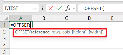
Diving into the syntax is like studying the blueprint for a machine. It’s essential to know which part goes where. The OFFSET function starts with a reference point, which is the cell or range from which it begins its journey. Then, you specify how many rows and columns to move from that initial point. Finally, you declare the height and width of the range you want to capture.
Here’s how it looks: =OFFSET(reference, rows, cols, [height], [width])
Each part plays a critical role:
- Reference: This is your starting block. Think of it as a home base.
- Rows: How many steps do you take up or down from your starting point?
- Cols: How many steps to the side, left or right, do you venture from home base?
- Height (optional): The size of the range you grab, measured in rows.
- Width (optional): The size of the range you grab, measured in columns.
By mastering the syntax, you craft the roadmap for your data journey, taking you from static to dynamic with grace and precision.
Constructing Dynamic Data Ranges
Basic Usage: Start Small, Think Big
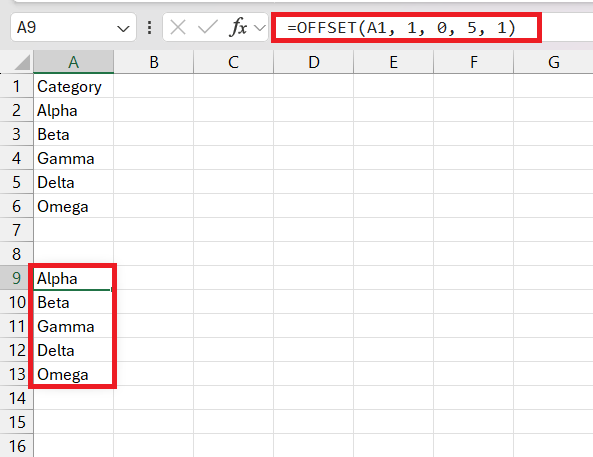
Begin your OFFSET journey with baby steps. Start by creating simple dynamic ranges that adjust as you add more data. In the most straightforward case, you might want to reference the five cells immediately below a starting cell (A1):
=OFFSET(A1, 1, 0, 5, 1)
This formula says, “Start at A1, go down one row, don’t go left or right, and give me a range that is five cells tall and one cell wide.” It results in a range from A2 to A6. Easy, right? Now imagine applying this to your monthly expense tracking: as you add more categories or months, your summary calculations can keep pace without constant tweaking. This is the ‘start small’ part.
The ‘think big’ piece comes with the understanding that these basic principles can be expanded to build highly complex, responsive spreadsheets. Once you’re comfortable with the easy stuff, scaling up to more advanced uses is a snap — and that’s where the real power lies.
Advanced Applications for Pro Users
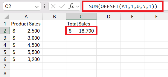
For the pros, OFFSET doesn’t just adjust; it transforms how you navigate data. Say you want to marry OFFSET with other functions. Need a dynamic range for your SUM formula? OFFSET can do that. How about variances between this quarter and the last? OFFSET’s got you covered.
=SUM(OFFSET(A1,1,0,5,1))
With OFFSET, you can do something like:
This formula dynamically adjusts to calculate the sum of the last N numbers in column A, regardless of how many new rows of data you add. Pro users leverage OFFSET in financial modeling, trend analysis, and real-time data visualization, creating documents that are as nimble as they are comprehensive.
Your spreadsheets stop being static tables and start becoming living entities that reflect the real-time ebb and flow of your data streams.
Tips to Avoid Common OFFSET Pitfalls
Steering Clear of Volatility Issues
One word of advice regarding OFFSET: it’s a volatile function, which means every time there’s a change in your workbook, it recalculates. And if it’s used excessively, this can slow things down. However, a little insider tip—most users don’t really encounter significant performance issues unless they really overdo it. You want to benefit from its dynamic powers without making Excel crawl at a snail’s pace.
It’s like adding hot sauce to a dish; just the right amount can take it to the next level, but overdo it, and you might regret it. So, use OFFSET judiciously, especially in large or complex spreadsheets. This way, you keep your data responsive without sacrificing the workbook’s performance.
Counteracting Limitations with Alternative Approaches
Every tool has its kryptonite, and OFFSET is no exception. For instance, when it turns your workbook into a sluggish beast, there are nifty alternatives to consider. One such superhero is the INDEX function, which, when combined with COUNTA, can construct dynamic ranges minus the volatility headaches.
Here’s a quick trick using INDEX instead of OFFSET: =SUM(INDEX($A$1:$A$100,1,1):INDEX($A$1:$A$100,COUNTA($A$1:$A$100)-1))
This alternative creates a dynamic range from the beginning of your data to the very last entry, without recalculating at every worksheet change. Such alternatives can keep workbooks efficient and responsive, proving that sometimes, a different tool can get the job done more effectively.
Going Beyond OFFSET: Integration with Other Functions
Synergizing OFFSET with MATCH for Precision
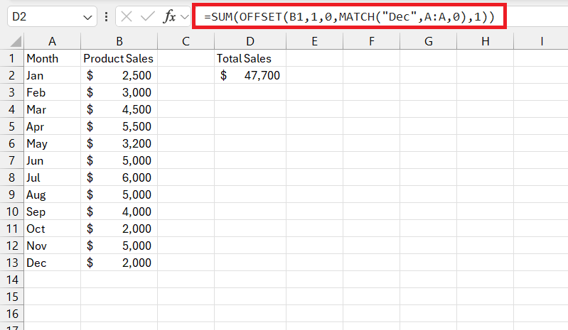
When you combine OFFSET with MATCH, you unlock a level of precision that can make your data analysis incredibly sharp. MATCH function scours through your rows or columns, seeking out a particular value and snagging its position. Pair that with OFFSET, and you’ve got a direct line to the exact data point you need, no matter where it’s positioned in your dataset.
It’s a bit like using a metal detector on a vast beach; MATCH finds the treasure, and OFFSET digs it up. The synergy between these two functions allows you to create lookup formulas that rival the likes of VLOOKUP or INDEX MATCH, but with an added layer of flexibility. Use them together, and you’ll pinpoint data points with the precision of a master marksman.
Pairing OFFSET with AVERAGE, MAX, MIN and SUM
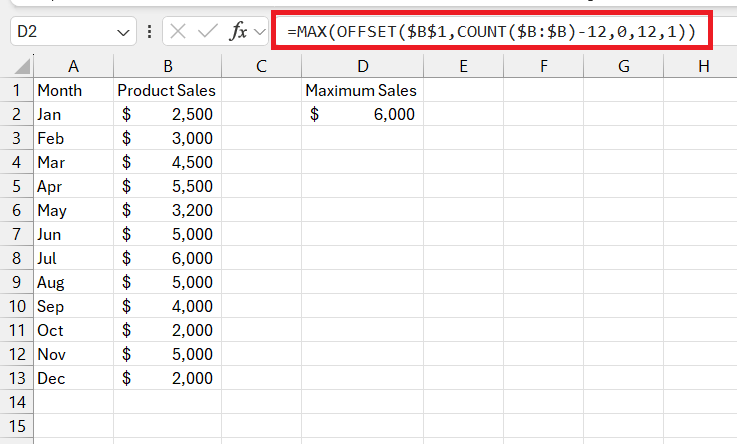
Taking OFFSET and marrying it with AVERAGE, MAX, MIN, or SUM turns it into a powerhouse for dynamic calculations. You can slice through a dataset, summarizing or analyzing only the pertinent bits. Let’s say you’re monitoring the peak performance of a sales team each month. Instead of tediously updating the range for MAX every time, you could use OFFSET to make it automatic:
=MAX(OFFSET($B$1,COUNT($B:$B)-12,0,12,1))
This gives you the maximum sales figure from the last 12 months, no matter how many rows of data you add each month. Pairing OFFSET with these statistical functions ensures your calculations remain up-to-date, hands-free. Whether you’re creating a moving average, tracking a rolling maximum, or calculating a dynamic sum, OFFSET in combination with these functions adjusts your formulas with the agility of a seasoned gymnast.
Frequently Asked Questions
What is the offset function in Excel used for?
The OFFSET function in Excel is used for creating dynamic cell references that can adjust automatically when data is added or removed. It’s especially useful for dynamic range calculations, creating flexible charts, and managing formulas that depend on changing data sets.
Can OFFSET Return a Single Value or an Entire Range?
Yes, the OFFSET function can return both a single cell value and an entire range of cells, depending on the height and width parameters you provide. If you set both to 1, you get a single cell; increase them, and you capture a larger range.
How Do I Create a Dynamic Named Range Using OFFSET?
To create a dynamic named range with OFFSET, define the starting cell, set rows and columns to 0, use COUNTA for the height to account for non-blank cells, and set width to 1:
=OFFSET(start_cell, 0, 0, COUNTA(column_range), 1)
What Are Some Alternatives to the OFFSET Function?
Some alternatives to the OFFSET function are INDEX with MATCH, INDIRECT for creating references as text, and dynamic array functions like FILTER and SORT available in the latest Excel versions.
What is the offset and match function in Excel?
The OFFSET function changes the reference point for a range, while MATCH searches for a specified item in a range and returns its position. Together, they create flexible, precise lookups in Excel, similar to INDEX MATCH.
John Michaloudis is a former accountant and finance analyst at General Electric, a Microsoft MVP since 2020, an Amazon #1 bestselling author of 4 Microsoft Excel books and teacher of Microsoft Excel & Office over at his flagship MyExcelOnline Academy Online Course.

